

The ability to lookup values is a MUST have skills for all Excel users. If you cannot lookup you cannot excel in data analysis.
In this article, I will show you 5 ways you can do a 2-way lookup in Excel.
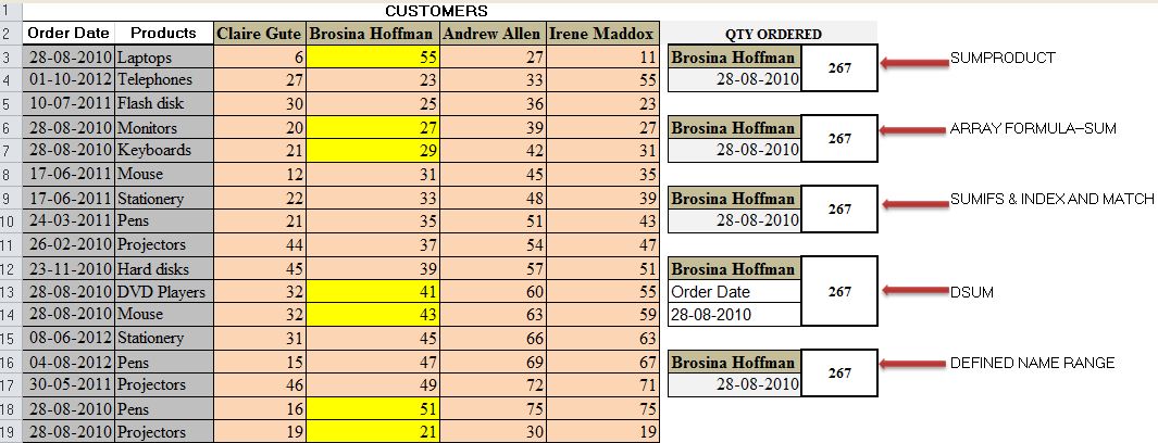
1. USING SUMPRODUCT
Using below sales data lookup and sum the total quantity for ALL items ordered by Brosina Hoffman on 28-08-2010?
=SUMPRODUCT((Order_dates=H4)*(Customers=H3)*Ordered_Quantity)=267
NB: Below are the references to the named ranges
Order_dates = A3:A19
Customers = C2:F2
Ordered_Quantity =C3:F19
How this works;
►(Order_dates=H4) creates a Boolean array showing TRUE for the Date criteria.
{TRUE;FALSE;FALSE;TRUE;TRUE;FALSE;FALSE;
FALSE;FALSE;FALSE;TRUE;TRUE;FALSE;FALSE;FALSE;TRUE;TRUE}
►(Customers=H3) creates a Boolean array showing TRUE for the Customer criteria.
{FALSE,TRUE,FALSE,FALSE}
►SUMPRODUCT converts the two Boolean arrays into its numeric equivalent of 1 & o and then using the techniques of the conjunction truth table, adds up the data in the intersections 55+27+29+41+43+51+21 = 267
How to get sum total orders for more than one customer?
What is the total quantity of ALL items ordered by Brosina Hoffman & Irene Maddox on 28-08-2010?
=SUMPRODUCT(((Customers=H4)+(Customers=H3))*(Order_dates=H5)*Ordered_Quantity)
The trick is including the 2 customers in the function
(Customers=H4)+(Customers=H3)–this ensures the two columns are dynamically selected.
{0,1,0,1}
2. USING ARRAY FUNCTION–SUM
{=SUM((Order_dates=H7)*(Customers=H6)*Ordered_Quantity)} =267
The array functions follow the same truth table logic. i.e. Forms a matrix where the criteria are met and multiplies it with ordered quantity matrix and sums the totals
3. SUMIFS, INDEX & MATCH
If you do not understand the logic in the conjunction truth table and you do not like array formulas then you can use SUMIFS, INDEX & MATCH
=SUMIFS(INDEX(Ordered_Quantity,,MATCH(H9,Customers,0)),Order_dates,H10)
How it works;
►INDEX(Ordered_Quantity,, MATCH(H9, Customers,0)) Selects the Column to sum dynamically. This provides SUMIF with a sum range
{55;23;25;27;29;31;33;35;37;39;41;43;45;47;49;51;21}
►SUMIFS takes in this Sum Range, filters it further using the Date criteria and then sums the array
4. DSUM
=DSUM(Data_Base,H12,H13:H14)=267
►Data_Base refers to the whole table from A2: F19–Includes the headings
How this works:
DSUM function sums the numbers in a column given the database it contains, column Position/Column Heading and a Criteria
DSUM( Data_base, Column_Heading, criteria )
5. DEFINED NAMED RANGES
=SUM(selected_orders)
The trick here is to first create a named range that will select the orders and then Sum the named range.
selected_orders= (Order_dates=$H$17)*(Customers=$H$16)*Ordered_Quantity
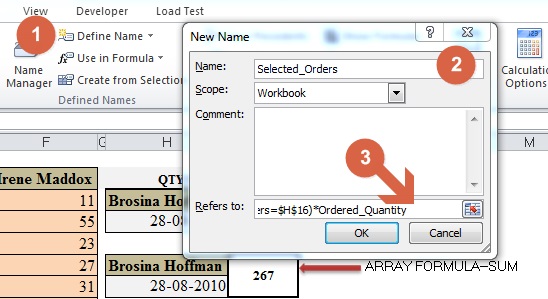
How to Create the Selected_Order Name Range
Go to Formulas►Define Name►Type the name you want►In the refers to section Paste your range (
(Order_dates=$H$17)*(Customers=$H$16)*Ordered_Quantity)
DOWNLOAD ABOVE EXAMPLE SPREADSHEET
RELATED ARTICLES


DSUM is the way to go. Most people ignore the all the “D” formulas which is a shame.
Thanks Kelvin. I think Database Functions are not that popular this is why they are mostly ignored.