How to Analyse Multiple Choice Survey Data In Excel

Knowing how to Analyse Multiple Choice Survey Data In Excel is a must-have skill since Multiple choice questions are the most popular questions.

For example, a Bank has requested it, customers, to rate 3 of its department’s services from Very Unsatisfied (-100%) to Very Satisfied (100%)

How do you convert the above data into the below graph?

There are 2 methods: Using Functions or Using Power Query

Using Formulas To Analyse Multiple Choice Survey Data In Excel

Step 1: Prepare the analysis section as shown below

Step 2: In cell G2, write this formula =(COUNTA(FILTER(FILTER($A$2:$C$17,$A$1:$C$1=$F3),FILTER($A$2:$C$17,$A$1:$C$1=$F3)=G$2))/16)*G$1

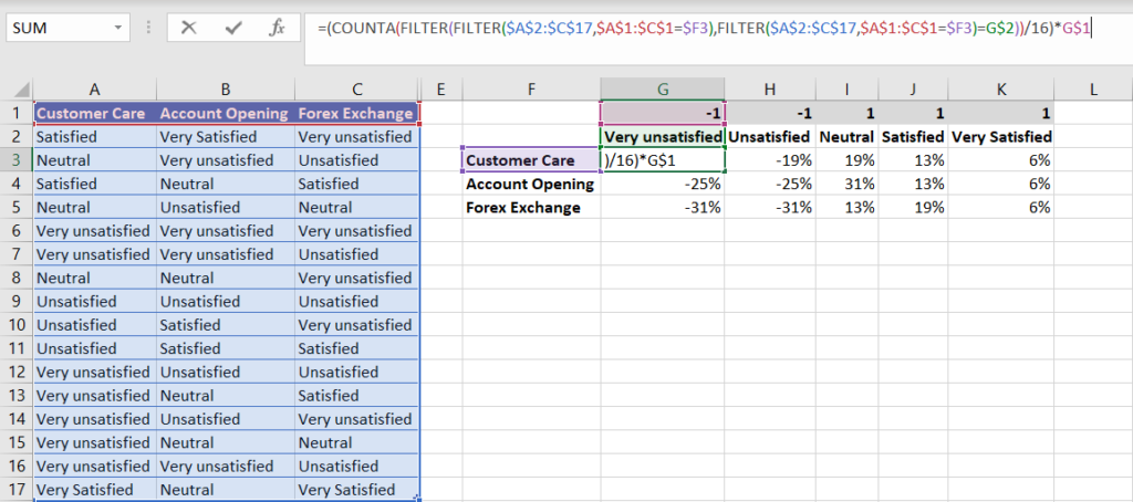
How the formula works:

Use the FILTER Function to get an array of responses per multiple choice and section, then count this array and divide by total responses to get the percent.

Multiply the percent by -1 for all unsatisfied/very unsatisfied customers and others by 1.

Insert graph and format as per liking.

Using POWER QUERY To Analyse Multiple Choice Survey Data In Excel

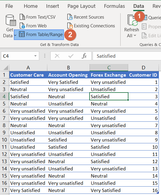
Step 1: Go to Data Tab, Click anywhere on the survey data table, and click From Table/Range

Step 2: On the power query editor, Select all the department columns, go to transform Tab, and click “Unpivot Columns”

Step 3: Click on Home Tab and click Close & Load

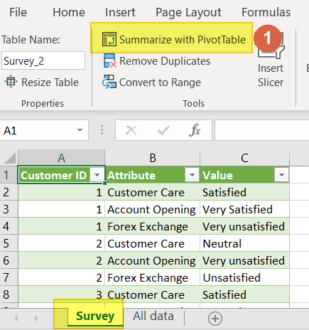
Step 4: When you close and load, a new worksheet is created containing a table of unpivoted data. Click Summarize with pivot table

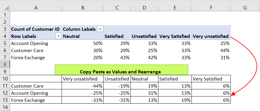
Step 5: In the Row field, place the departments, in the Column Field, place the responses, and in the Value setting, Place the Customer ID.

NB: Edit the Value Field setting to count and Show values as % of Parent Row Total

Step 6: Copy & Paste Pivoted table as Values, and rearrange them as shown below. Finally, insert and format the graph using this data

Conclusion:

Power Query option is the most versatile option but with numerous steps.

DOWNLOAD WORKSHEET

Reference:

How to Analyze Survey Data in Excel + Video