IF function is one of the most used functions in Excel.

In my opinion, it is the foundation of all programming and Excel formulae mastery.  

However, it is also one of the most misused functions, especially Nested IF.

Especially now with Excel 2007 and beyond, you can nest up to 64 IF functions to form complex, slow, and hard-to-understand IF then ELSE statement.

You don’t need to slow or complicate your worksheet anymore, here are the 14 faster alternatives:

NESTED IF

Say you have below price list with mixed currency and you want to convert them to USD

The first step would be to look up the exchange rate per currency. Most users would use the below nested IF function

=IF(B2=$F$3,$G$3,
   IF(B2=$F$4,$G$4,
    IF(B2=$F$5,$G$5,
      IF(B2=$F$6,$G$6,
        IF(B2=$F$7,$G$7,
          IF(B2=$F$8,$G$8))))))

This is not only hard to understand but will definitely slow down your worksheet.

NB:

• Nested IF forms the Value_if_False of the previous IF function
• Watch out for the closing parenthesis!
• If your test values are hierarchically related, start the test with the highest value since Nested IF returns the 1^st TRUE test
• If all logical tests result in FALSE and the default Value-if-False function is given, the function returns FALSE.

VLOOKUP

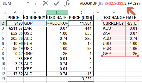
=VLOOKUP(B2,$F$2:$G$8,2,FALSE)

How it works

VLOOKUP Function uses the exact match criteria to retrieve the exchange rates in Column 2 of the exchange rate table ($F$2:$G$8).

Note: You MUST specify the match criteria for VLOOKUP to exactly retrieve the correct rates. If the criterion is omitted, VLOOKUP, by default, does an approximate search giving wrong results.

One of the situations where you want VLOOKUP using an approximate match is where your test values are hierarchically related.

For example, you want to look up the discount percentage based on the sales value

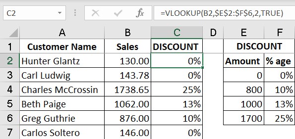
How the Formula Works

VLOOKUP compares sales with the amount in the discount table.

If sales are equal to or greater than the discount amount, it returns the corresponding percentage, otherwise, it looks at the next lesser amount percentage.

Read more on VLOOKUP Function

CHOOSE & MATCH FUNCTIONS

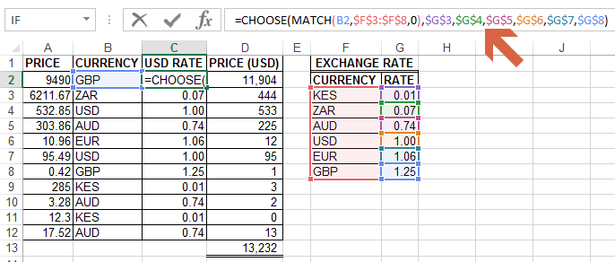
=CHOOSE(MATCH(B2,$F$3:$F$8,0),$G$3,$G$4,$G$5,$G$6,$G$7,$G$8)

How it works

MATCH(B2,$F$3:$F$8,0)=6

MATCH function searches for the currency in the exchange rate table and returns its relative position.

CHOOSE function returns the exchange rate based on its position in the list. MATCH function above provides this position.

=CHOOSE(6,$G$3,$G$4,$G$5,$G$6,$G$7,$G$8) = 1.25

REPT FUNCTION

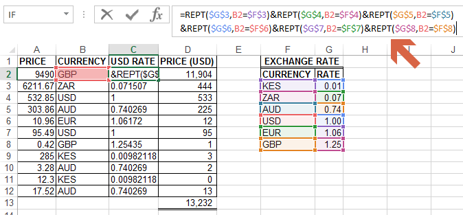
=REPT($G$3,B2=$F$3)&
REPT($G$4,B2=$F$4)&
REPT($G$5,B2=$F$5)&
REPT($G$6,B2=$F$6)&
REPT($G$7,B2=$F$7)&
REPT($G$8,B2=$F$8)

How It Works

REPT Function returns a specific text string a specified number of times. If the specified number is zero, REPT returns an empty string.

Internally, Excel recognizes the value of TRUE as 1 and the value of FALSE as 0. This is a fact that REPT utilizes to determine the number of times to repeat.

Also, note that in our function above ONLY 1 test will evaluate TRUE, others return FALSE.

=REPT($G$3,FALSE)&REPT($G$4,FALSE)&REPT($G$5,FALSE)
&REPT($G$6,FALSE)&REPT($G$7,FALSE)&REPT($G$8,TRUE)

Where the test evaluates to FALSE, REPT functions return an empty string (” “)

=""&""&""
&""&""&"1.25435"

Read more on REPT Function

INDEX & MATCH

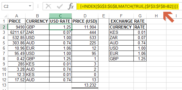
{=INDEX($G$3:$G$8,MATCH(TRUE,($F$3:$F$8=B2),0))}

How it works

MATCH function checks if the currency exists in the range ($F$3:$F$8=B2). If TRUE, it returns the relative position of the currency.

The INDEX function returns the exchange rate in the range ($G$3:$G$8) given its position. MATCH provides this relative position.

NB: This is an array formula, Therefore, Ctrl+Shift+Enter

If want to avoid the array formula, use a combination of INDEX, MATCH, and INDEX shown below

=INDEX($G$3:$G$8,MATCH(TRUE,INDEX($F$3:$F$8=B2,0),0))

Based on the comment below by Keith, I have realized the above INDEX & MATCH function is overkill and simple INDEX & MATCH below works perfectly and much faster than the above combinations.

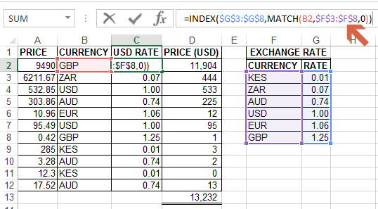
=INDEX($G$3:$G$8,MATCH(B2,$F$3:$F$8,0))

SUMPRODUCT

=SUMPRODUCT(--(B2=$F$3:$F$8),$G$3:$G$8)

How it works

In my opinion, this is the shortest and efficient formula.

►–(B2=$F$3:$F$8) returns an array of 1/0.     {0;0;0;0;0;1}

1 representing the relative position of the currency that meets the criteria in the exchange rate table

►$G$3:$G$8 returns an array of exchange rates  {0.00982118;0.071507;0.740269;1;1.06172;1.25435}

SUMPRODUCT gets the sum of the product of the two arrays

=SUMPRODUCT({0;0;0;0;0;1},{0.00982118;0.071507;0.740269;1;1.06172;1.25435})=1.25435

NB: This method ONLY  works with numeric values.

BOOLEAN LOGIC

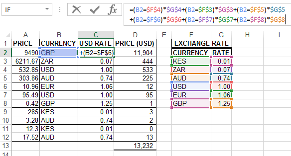
=(B2=$F$4)*$G$4+(B2=$F$3)*$G$3+(B2=$F$5)*$G$5
+(B2=$F$6)*$G$6+(B2=$F$7)*$G$7+(B2=$F$8)*$G$8

How it works

The method exploits the fact that internally, Excel recognizes the value of TRUE as 1 and the value of FALSE as 0.

Firstly, Compare the currency in the price list table with the currency in the exchange rate.  This results in TRUE/FALSE which Excel recognizes as 1/0.

=(0)*$G$4+(0)*$G$3+(0)*$G$5
+(0)*$G$6+(0)*$G$7+(1)*$G$8

Since only 1 test will evaluate to TRUE, if you multiply them with corresponding  rates and add them up, the result will be zeros plus the correct rate

=0+0+0
+0+0+1.25435

NB: This method also ONLY  works with numeric values.

SUMIF

How it works

This is another simple alternative but works ONLY with numeric values.

SUMIF function returns a sum of all numbers in a range of cells that meet a certain criterion.

syntax =SUMIF(Range, Criterion, [sum_range])

Range–Currencies to be evaluated using our criterion

Criterion–the currency on our price list that determines the exchange rate to be returned

Sum_range–the exchange rates

Since only one cell in our range will meet our criterion, SUMIF returns the coinciding rate.

IFS FUNCTION

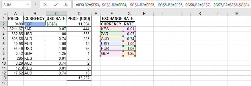
=IFS(B2=$F$3, $G$3,
      B2=$F$4, $G$4,
       B2=$F$5, $G$5,
        B2=$F$6, $G$6,
         B2=$F$7, $G$7,
          B2=$F$8, $G$8)

This is a simplified Nested IF since you do not need to retype the IF function with every logical test–all you need is to type the logical test and its value if True.

Things to note on the IFS function:

• It evaluates up to 127 different conditions.
• It Returns the Value for the 1st Logical test that evaluates into TRUE
• Where there is no corresponding value_if_true, the function displays the message “You’ve entered too few arguments for this function”.
• If logical test does not result in TRUE/FALSE, the function returns #VALUE! error.
• If all logical tests result in FALSE, the function returns #N/A error.

To resolve the #N/A error, always end your function with TRUE, then value to return if all else is false.

i.e., =IFS(logical_test1, value_if_true1, [logical_test2, value_if_true2]…TRUE, 0)

• Found from Excel 2019 greater versions.

SWITCH FUNCTION

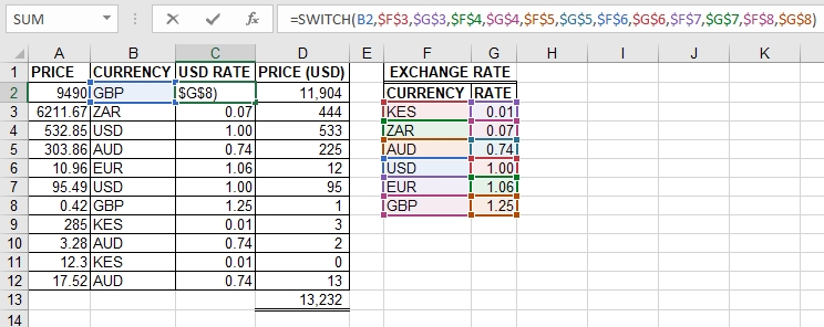
=SWITCH(B2,$F$3,$G$3,$F$4,$G$4,$F$5,$G$5,$F$6,$G$6,$F$7,$G$7,$F$8,$G$8)

This Video best explains how the SWITCH Function works

Things to note on the SWITCH function:

• It Returns the result of the 1st Match between Value & Expression.
• The expression can be a Value, Boolean(True/False), or a Function.
• Matching values and corresponding results are entered in pairs.
• Can handle up to 126 pairs.
• Always include the last Default value if no match is found to avoid the #N/A error.
• Only performs an exact match, so you cannot use (>, <).

So, use TRUE as an expression and use a formula that evaluates TRUE

i.e =SWITCH( TRUE, a>b, xu, c<=y, zb, TRUE, gh)

• Found from Excel 2019 greater versions.

MAXIFS/MINIFS

MAXIFS/MINIFS functions return the maximum or minimum number in a range that meets a criterion.

This only works for numeric data.

AVERAGEIFS

This function calculates the average of numbers in a range that meets one or more supplied criteria.

XLOOKUP

Read More on how XLOOKUP function works

FILTER FUNCTION

Read More on how FILTER Function Works

DOWNLOAD WORKSHEET 

RELATED ARTICLES

7 OVERLOOKED USES OF EXCEL MOD FUNCTION

EXCEL’S WEEKDAY FUNCTION IN-DEPTH

RESOURCES

This article was inspired by the Excel Hero epic article  I Heart IF.

Check it out and ensure you read all 100+ comments

RECOMMENDED BOOKS

EXCEL OUT-OF-BOX CREATIVITY BOOKS